Path Tracing Foundations: A Mathematical Overview

Understanding path tracing from equations.

Introduction

Rendering is a broad term describing a collection of image synthesis techniques that takes geometrical descriptions and material properties of a 3-D scene as input, and outputs a 2-D image of that scene from a specific point of view. In layman’s terms, it is like taking a photograph, except the scene and the camera are both computer simulated. The rendering equation (or light transport equation, LTE) proposed by Kajiya¹ is as follows:

\[L_{o}\left(p, w_{o}\right)=L_{e}\left(p, w_{o}\right)+\int L_{i}\left(p, w_{i}\right) f\left(p, w_{i}, w_{o}\right) \cos \theta_{i} d w_{i},\]

Where \(L_{o}\) is the outgoing radiance along direction \(w_{o}\) originated at point \(p\), and \(L_{e}\) is the emitted radiance. Followed is an infamous integral which is extremely hard to solve since the whole LTE is a recursive equation. The integration involves integrating over all incoming radiance multiplied by a special quantity \(f\left(p, w_{i}, w_{o}\right)\) commonly known as BSDF (bi-directional scattering distribution function). Recursively expand the LTE and using \(p\) plus an arrow to represent both position and direction, we get

\[\begin{split} L_{o} & \left(p_{1} \rightarrow p_{0}\right) = L_{e}\left(p_{1} \rightarrow p_{0}\right) \\ & + \int L_{e}\left(p_{2} \rightarrow p_{1}\right) f\left(p_{2} \rightarrow p_{1} \rightarrow p_{0}\right) \cos \left(\theta_{1}\right) d w_{1} \\ & + \int \int L_{e}\left(p_{3} \rightarrow p_{2}\right) f\left(p_{3} \rightarrow p_{2} \rightarrow p_{1}\right) \cos \left(\theta_{2}\right) f\left(p_{2} \rightarrow p_{1} \rightarrow p_{0}\right) \cos \left(\theta_{1}\right) d w_{2} d w_{1} \\ & + \cdots \end{split}\]

which is clearly an infinite-dimensional integral that is really unlikely to have an analytical solution. Techniques like Bi-directional Path Tracing (BDPT), Metropolis Light Transport (MLT), Photon Mapping, Vertex Connection and Merging (VCM) are already proven to be quite effective in solving the LTE, but any of them can be hard to done right without previous experiences. The most basic form of path tracing and be further categorized into 4 different kinds of integration/rendering techniques. I have implemented all of them from scratch as the fundamental building block for advanced techniques (as well as to verify the results of other techniques). Implemented techniques including

Vanilla Path Tracing

Tracing rays starting at the camera; rays reflect and refract and collect intersection information until an emitter is found. This is the most frequently seen algorithm from online tutorial or elementary rendering courses. This method is unbiased, consistent, but can be slow to converge in most cases.

Backward Light Tracing

Similar to the aforementioned one, this algorithm is unbiased and consistent. By splitting radiance contribution into direct and indirect parts, we can directly sample the light at each intersection point. Obviously this technique is especially suitable for scenes with small light sources. Sometimes this technique is also called “path tracing with next event estimation”.

MIS’ed Path Tracing

Vanilla Path Tracing (VPT) and Backward Light Tracing (BLT) both have their weaknesses. The former one is good at handling specular surfaces and large light sources, while the later one is good at handling diffusive surfaces and small light sources. Can we combine them in an unbiased & consistent way? Veach’s legendary doctoral thesis² proposed a method called Multiple Importance Sampling (MIS) came to the rescue.

Light (Particle) Tracing

This method is also unbiased and consistent and can be tricky to implement. Using Veach’s naming convention: \(s\) stands for path vertices staring from the emitter, \(t\) for path vertices starting from the camera, light tracing is essentially a \(s=n\), \(t=1\) sampling technique of Bi-directional Path Tracing. Interestingly, although many documents mentioned Light Tracing (LT), neither a detailed algorithm description nor a publicly available implementation can be easily found. To my knowledge, my implementation is the second open source Light Tracing integrator.

The following paragraphs will describe how each technique is implemented.

Pre-requirements

Since I am implementing these rendering techniques from scratch, the architecture of the renderer must be carefully designed. Inspired by PBRT version 2 and 3³, Mitsuba⁴, LuxRender⁵, and Tungsten⁶ (along with some previous experience on the Java based Photon-v1), I chose the powerful C++ as the main programming language for Photon-v2. I later combined the cosine term in the LTE with BSDF into an abstract base class called BSDFcos, each implementation must provide an evaluation, an importance sampling and a method for PDF querying. For evaluating the effectiveness of different rendering methods, the classic Lambertian diffuse BRDF and microfacet based BSDF materials are also implemented. Unfortunately, the paper by Walter et al.⁷ contains several errata and some of them got “lucky” enough to confuse me quite a bit. A suitable mapping function from roughness to GGX alpha is not provided in the paper either (luckily PBRT-v3 provided such mapping equation but did not mention how it was derived). My choice of acceleration structure is k-D tree with SAH based subdivision strategy (for testing these rendering methods). In the system I designed, camera and emitter implementations must provide several sampling methods which are essential for the following integration techniques.

Vanilla Path Tracing

Recursively expand the LTE like how it is done in the introduction section, we got a general representation for the \(n\)th integral:

\[T \left(n\right) = \int {\cdots \atop n} \int L_{p}\left(p_{n+1} \rightarrow p_{n}\right) \cdot \prod_{i=1}^{n}\Big[f\left(p_{i+1} \rightarrow p_{i} \rightarrow p_{i-1}\right) \cos \left(\theta_{i}\right)\Big] d \omega_1 d \omega_2 \cdots d \omega_n\]

Now we can write the LTE with infinite number of expansions as:

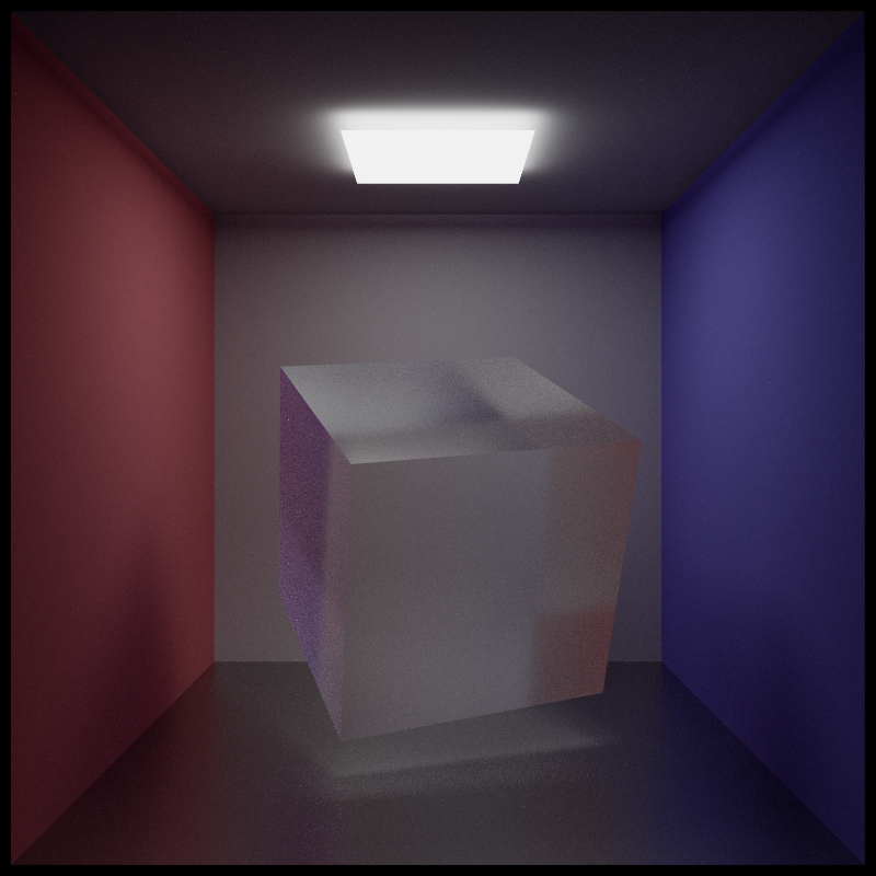
\[L_{o} \left(p_{1} \rightarrow p_{0}\right) = L_{e} \left(p_{1} \rightarrow p_{0}\right) + \sum_{n=1}^{\infty} T \left(n\right)\]

Quite an elegant form, isn’t it? If you are interested in a more in-depth explanation, be sure to pay a visit to Jiayin Cao’s blog⁸ where I learned much of the basic concepts from. Apart from the direct (zero bounce) illumination term \(L_{e} \left(p_{1} \rightarrow p_{0}\right)\), each term in the summation represents an integral over \(n\) dimensional space. In order to get a reasonable converging rate, Monte-Carlo based integration method is used. Notice that there is no need to generate each path from scratch: by using Russian-Roulette (RR) path terminating technique, if a path terminates at camera vertex \(t = i\), one can evaluate the integrand of \(T \left(1\right)\), \(T \left(2\right)\), \(\cdots\) to \(T \left(i - 1\right)\). The source code for integration is located at “Source/Core/Integrator/BackwardPathTracing.cpp”. The correctness of this integration method is verified since some rendered results have been compared to my Java-based renderer which was previously compared to PBRT-v2 and had no differences at all. Following is a rendered image of a simple Cornell Box scene using this technique:

Backward Light Tracing

Also known as path tracing with next event estimation, this technique works by first formatting the LTE into two parts

\[L_{o} \left(p_{1} \rightarrow p_{0}\right) = L_{e} \left(p_{1} \rightarrow p_{0}\right) + L_{r} \left(p_{1} \rightarrow p_{0}\right).\]

Substituting back into the LTE, we have

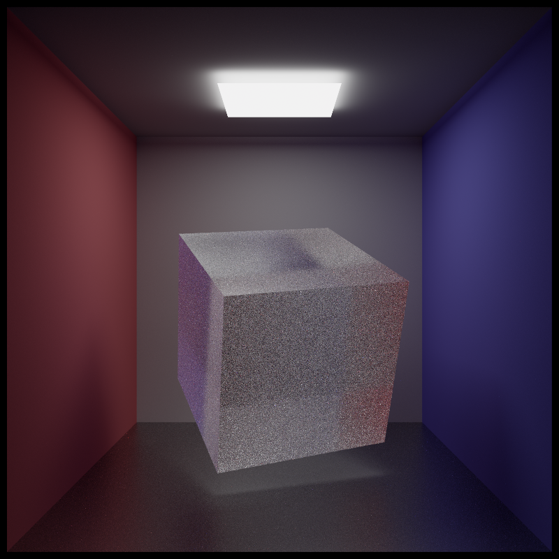
\[\begin{split} L_{o} \left(p_{1} \rightarrow p_{0}\right) \\ = & L_{e} \left(p_{1} \rightarrow p_{0}\right) \\ & + \int \Big[ L_{e} \left(p_{2} \rightarrow p_{1}\right) + L_{r} \left(p_{2} \rightarrow p_{1}\right)\Big] f\left(p_{2} \rightarrow p_{1} \rightarrow p_{0}\right) \cos \left(\theta_{1}\right) d \omega_1 \\ = & L_{e} \left(p_{1} \rightarrow p_{0}\right) \\ & + \int L_{e} \left(p_{2} \rightarrow p_{1}\right) f\left(p_{2} \rightarrow p_{1} \rightarrow p_{0}\right) \cos \left(\theta_{1}\right) d \omega_1 \\ & + \int L_{r} \left(p_{2} \rightarrow p_{1}\right) f\left(p_{2} \rightarrow p_{1} \rightarrow p_{0}\right) \cos \left(\theta_{1}\right) d \omega_1 \\ = & L_{e} \left(p_{1} \rightarrow p_{0}\right) + L_{d} \left(p_{2} \rightarrow p_{1} \rightarrow p_{0}\right) + L_{i} \left(p_{2} \rightarrow p_{1} \rightarrow p_{0}\right), \end{split}\]

where \(L_d\) is the direct term and \(L_i\) is the indirect term. Recursively expand the above equation, we can arrive at a similar formula as Vanilla Path Tracing for next event estimation. Those integrals told us that if the shape of the integral is dominated by the \(L_d\) term, i.e., small light sources like a point light, this technique can have vast amount of advantages over Vanilla Path Tracing. But it is quite inefficient with scenes lit mainly by caustics since transparent objects served as occluders for light sources. As usual, the rendering equation is solved with Monte-Carlo (MC) and RR techniques (and the source code is located at “Source/Core/Integrator/BackwardLightTracing.cpp” if you want to take a look). Here is the same Cornell Box scene rendered using this technique:

One thing worth noting is that if the ray for indirect lighting randomly hit an emitter, its contribution should not be counted, otherwise the scene will be two times brighter since we already sampled it using the direct lighting term.

MIS’ed Path Tracing

In the previous rendering algorithm, if we randomly hit an emitter, its contribution should be ignored. This sounds like a waste, but can be cured by a simple yet powerful technique called Multiple Importance Sampling (MIS). The multi-sample estimator proposed by Veach is as follows:

\[F = \sum_{n=1}^{n} \frac{1}{n_i} \sum_{j=1}^{n_i} W_i \left(X_{i,j}\right) \frac{f\left(X_{i,j}\right)}{p_i\left(X_{i,j}\right)}\]

where \(p_i\left(X_{i,j}\right)\) is the probability density of choosing a sample \(X_{i,j}\) and \(i\) techniques are combined using weighted sum. The weighting function \(W_i \left(X_{i,j}\right)\) can be a per-sample weighting and the result is guaranteed to be unbiased if several conditions are met (not listed here). Several weighting heuristic are provided with Veach’s thesis², and my choice is the power heuristic with \(\beta=2\), which is also the choice of PBRT, Mitsuba and LuxRender:

\[W_i = \frac{p_i^\beta}{\sum_k p_k^\beta}.\]

With \(\beta=2\), the weighting is “sharpened” and works pretty well in most situations. A sample will have low weighting factor when the “confidence” of taking that path is low (low PDF, may induce fireflies); if the sample has high PDF, a large weighting factor is used. This technique greatly lower the variance of a rendering process. In order to implement MIS combining Vanilla Path Tracing and Backward Light Tracing, a separate interface for querying PDF is essential for both BSDFcos (see “Source/Core/SurfaceBehavior”) & Emitter (see “Source/Core/Emitter”) implementations. Following is the Cornell Box scene rendered using MIS technique:

Light (Particle) Tracing

This method utilizes the adjoint of radiance, importance, for rendering. To implement this technique, we must rewrite the LTE in surface form

\[L_{o} \left(p_{1} \rightarrow p_{0}\right) = L_{e} \left(p_{1} \rightarrow p_{0}\right) + \int L_{i} \left(p_{2} \rightarrow p_{1}\right) f \left(p_{2} \rightarrow p_{1} \rightarrow p_{0}\right) G \left(p_{2} \leftrightarrow p_{1}\right) d A_1,\]

where \(G \left(p_{2} \leftrightarrow p_{1}\right)\) stands for geometry term and \(V \left(p_{2} \leftrightarrow p_{1}\right)\) is the visibility test:

\[G \left(p_{2} \leftrightarrow p_{1}\right) = V \left(p_{2} \leftrightarrow p_{1}\right) \frac{\vert \cos \left(\theta_{1}\right) \cos \left(\theta_{2}\right) \vert}{\vert p_2 - p_1 \vert^2}\]

Veach also introduced another equation called the measurement equation:

\[I = \int_{A_{lens}} \int_{A_{film}} W_e\left( p_{film} \rightarrow p_{lens} \right) L\left( p_{film} \rightarrow p_{lens} \right) G\left( p_{film} \rightarrow p_{lens} \right) dA_{film} dA_{lens}\]

where \(W_e\) is a quantity that transform the measured power into radiance, which we named “importance” (this is easy to confuse with importance-sampling, the word importance have different meaning there). When we plug the surface form LTE into the measurement equation and recursively expand it, something amazing happened

\[\begin{split} I = & \sum_{k=1}^{\infty} \int_{A^{k+1}} L_{e} \left(p_{1} \rightarrow p_{0}\right) G \left(p_{1} \leftrightarrow p_{0}\right) \\ & \cdot \prod_{i=1}^{n} \left[ f \left(p_{i-1} \rightarrow p_{i} \rightarrow p_{i+1}\right) G \left(p_{i} \rightarrow p_{i+1} \right) \right] W_e\left( p_{k-1} \rightarrow p_{k} \right) dA_0 dA_1 \cdots dA_k. \end{split}\]

The importance, \(W_e\), can be transported like an emitted quantity just like \(L_e\)! Also the integration over each differential area is order independent. To implement light tracing, we shoot rays from the emitter, reflect and refract depend on the surfaces they hit. An additional visibility test is done between each intersection point and the camera, then we solve the above equations using MC and RR. This light tracing integration technique is equivalent to the \(s=n\), \(t=1\) style Bi-directional Path Tracing. The following image is also the same Cornell Box scene rendered using this technique:

Results and Comparisons

All images are rendered using Intel i7 3770 CPU with 8 threads. No post-processing is involved except a tone-mapping operator (proposed by Jim Hejl and Richard Burgess-Dawson at GDC) is applied in order to view the images on normal monitors.

Put the simple Cornell Box renderings from above sections closely:

From left to right: vanilla path tracing, backward light tracing, MIS'ed path tracing, light tracing

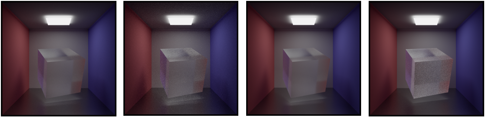
Clearly, they all tend to converge to the same result, despite some of them have fireflies in specific regions. All the above images are rendered with roughly same amount of time. light tracing works very well on every region except on the glass cube. My guess is that since an explicit connection between the intersection point and the camera must be established for the radiance to come through, inside transparent objects, there are occluders everywhere and visibility tests would certainly fail; occasionally, a ray survived the RR and got the chance to have valid camera connection, which leads to high variance. MIS’ed path tracing works the best among 4 methods, and vanilla path tracing also doing pretty well due to the not-so-small light source located just below the ceiling.

Another test scene is far more interesting. I simulate water with several superpositioned spatial sine and cosine functions, discretize the result into a height field, and use the smooth shading algorithm from the first course assignment to make it appear to be continuous. Filling the Cornell Box with simulated water and place a submerged Stanford Dragon and lit by a small area light, the following images are rendered with roughly 3 hours of time (at 800x800 resolution):

Vanilla path tracing

Backward light tracing

MIS'ed path tracing

Light tracing

Reference Image (MIS’ed path tracing, 18 hours of rendering, 16000spp)

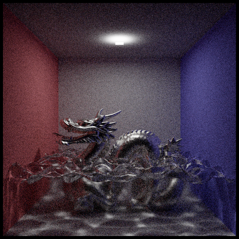
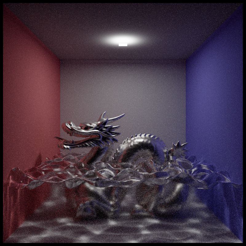
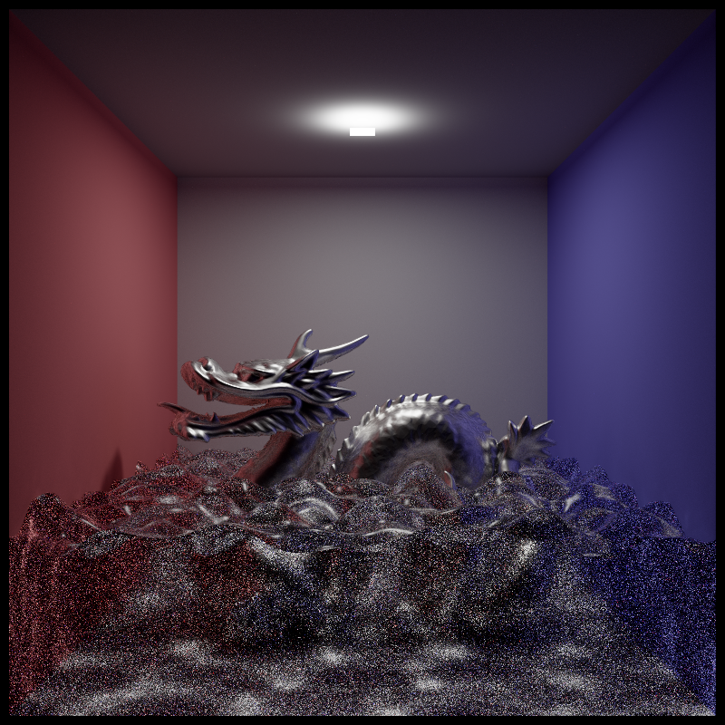
Unsurprisingly, vanilla path tracing handles small light sources badly which results in high variance; MIS’ed path tracing has the clearest caustics among 4 methods; light tracing performs poorly in underwater regions due to the same reason mentioned before.

In conclusion, I would say that MIS’ed path tracing has the best performance both visually and theoretically, and light tracing has the largest potential since it can be extended into BDPT. Vanilla path tracing and backward light tracing can be used for reference image rendering since their implementations are far more straightforward compare to the rests and should be less prone to bugs.

The following images are rendered purely for artistic reasons. An area light using a beautiful image as its radiance map and illuminates the chromium Stanford Dragon submerged in my simulated water domain:

MIS’ed path tracing, 8 hours at 800x800 pixels, 5000spp

Glass Stanford Dragon (MIS’ed PT, 8 hours at 800x800 pixels, 6000spp)

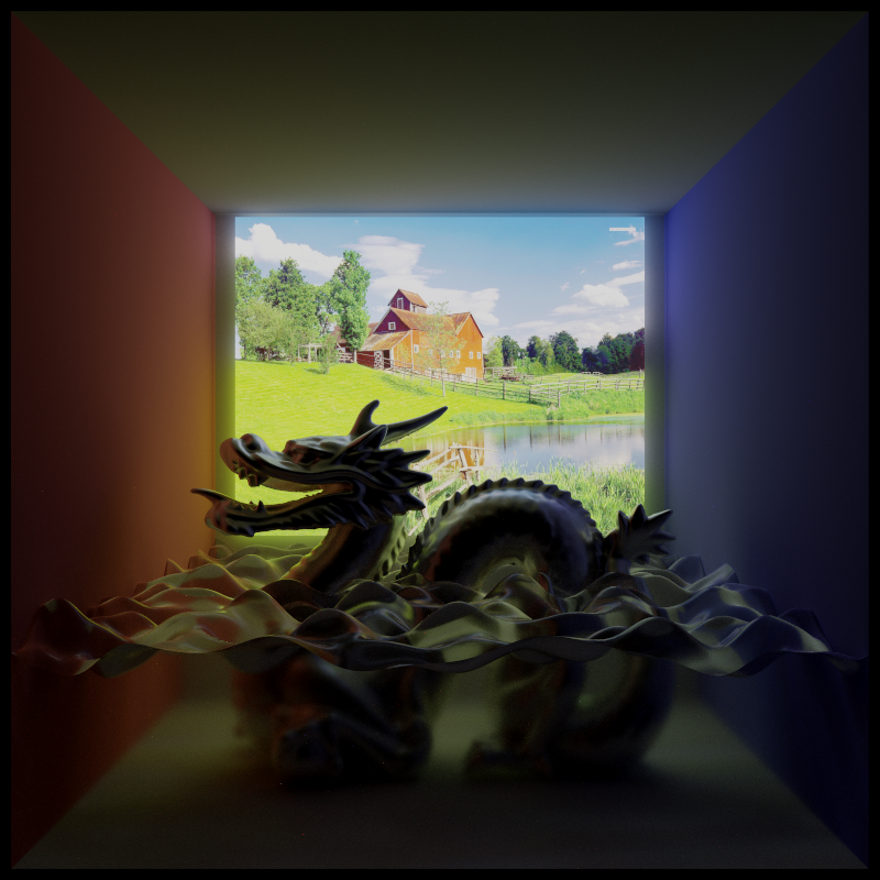
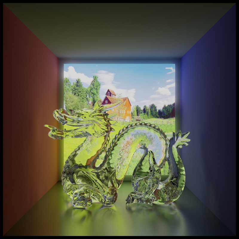
Implementing these rendering algorithms can be really useful if I later decided to implement BDPT, MLT or novel integration algorithms like VCM. Being impressed by the amount of math involved and how elegantly they were formulated, it sure has worsened my long-time addition to computer graphics…

Footnotes

1. J. T. Kajiya, “The rendering equation”. SIGGRAPH 1986. ↩

2. E. Veach, “robust monte carlo methods for light transport simulation,” 1997. ↩ ↩²

3. Matt Pharr, Wenzel Jakob, Greg Humphreys, “Physically Based Rendering 3rd Edition”. ↩

4. W. Jakob, “Mitsuba Renderer (http://www.mitsuba-renderer.org/)”. ↩

5. LuxRender (http://www.luxrender.net/). ↩

6. B. Bitterli, “Tungsten Renderer (https://benedikt-bitterli.me/tungsten.html)”. ↩

7. B. Walter, “Microfacet Models for Refraction through Rough Surfaces”. ↩

8. A Graphics Guy’s Note (https://agraphicsguy.wordpress.com/). ↩